Streaming 101

What is streaming?

Streaming system: A type of data processing engine that is designed with infinite datasets in mind.

Two dimensions to describe a dataset:

• Cardinality
  • Dictates the dataset size.
  • Bounded/unbounded.
• Constitution
  • Dictates the physical manifestation: the ways one can interact with the data in question.
    • Table
      • A holistic view of a dataset at a time point.
      • SQL
    • Stream
      • Element-by-element view of the evolution of a dataset over time.

Greatly exaggerated limitations of streaming

• Streaming systems have historically been relegated to a somewhat niche market of providing low-latency, inaccurate or speculative results. (Lambda architecture)
• Kappa architecture: Run a single pipeline that can replay.
• A well-designed streaming system actually provide a strict superset of batch functionality. (Apache Flink)

Streaming systems need two things to beat batch ones:

• Correctness
  • Boils down to consistent storage.
  • Streaming systems need a method for checkpointing persistent state over time, which should remain consistent in light of failures.
    • Strong consistency is required for exact-once processing.
      • (ST) Strong consistency -> unique ID -> exact-once -> correctness.
• Tools for reasoning about time
  • Essential for dealing with unbounded, unordered data of varying event-time skew.

Event time vs. processing time

Two domains of time:

• Event time
  • When the event actually occurred.
• Processing time
  • When the event is observed in the system.

The skews between event time and processing time are often highly variable.

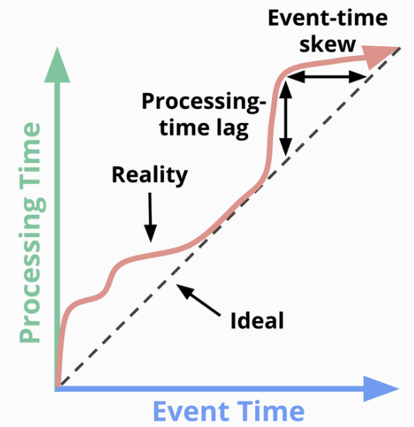
Processing-time lag is always equal to event-time skew.

Windowing:

• By processing time: not quite make sense if we care about event time, since some events may fall into wrong processing-time window due to skew.
• By event time: Need a way to reason the completeness, how we can determine when we have observed all events in a window.

Data processing patterns

Bounded data

The overall model is quite simple, using engines like MapReduce.

Unbounded data: batch

Batch engines can be used to process unbounded data by windowing.

• Fixed windows
  • Process each window as a separate, bounded data source.
  • Completeness problem: Some events may be delayed.
• Sessions
  • A period of activity terminated by a gap of inactivity.
  • Not ideal since a session may be split across batches.

Unbounded data: streaming

Unbounded data sources in reality may be high unordered with respect to event times, or of varying event-time skew. 4 groups of approaches can help:

• Time-agnostic
  • Used when time is essentially irrelevant.
  • Engines just need to support basic data delivery.
  • Examples
    • Filtering, e.g., web log for a specific domain.
    • Inner joins: buffer the inner source and check the events from the other source.
      • May be time-related if we want garbage collection.
• Approximation
  • Algorithms: approximate Top-N, streaming k-means etc.
  • Designed to be low overhead but limited and often complicated.
  • Usually processing-time based and provides some provable error bounds on the approximations.
• (Windowing basics)
  • Fixed windows, tumbling, no overlap
  • Sliding windows, hopping, with overlap
  • Sessions
• Windowing by processing time
  • Nice things
    • Simple.
    • Judging window completeness is straightforward.
    • Exact what we want if we want to infer information as the data is observed. e.g., monitoring.
  • Downside
    • Cannot reflect the reality in event time domain. Processing-time order doesn’t respect event-time order.
• Windowing by event time
  • Supports for it has been evolving: Flink -> Spark -> Storm -> Apex.
  • Advantages
    • Gold standard of windowing.
    • Correctness
    • Dynamically sized windows like sessions.
  • Problems
    • Buffering: more buffering is required
      • Good things
        • Persistent storage is cheaper now.
        • Update can be incremental, without buffering entire input set.
    • Completeness
      • No good way of knowing when we’ve seen all of data for a given window.
      • Solution: Use heuristic estimate like watermarks (MillWheel, Cloud Dataflow, Flink).
        • If we need absolute correctness, The only real option is let the pipeline builder to express when to materialize.

The What, Where, When and How of data processing

Roadmap

Five main concepts for this chapter:

• Processing time vs. event time
  • Use event time if we care about correctness and when things actually occur.
• Windowing
  • Fixed, sliding, sessions.
• Triggers
  • A mechanism for declaring when the output for a window should be materialized relative to some external signal.
  • Can have multiple triggers to observe the output for a window multiple times as it evolves. (early update, processing late data)
• Watermarks
  • A notion of input completeness with respect to event times.
  • Statement for a watermark with value of time X: All input data with event times less than X have been observed.
• Accumulation
  • Specify the relationship between multiple results that are observed for the same window.
  • Different accumulation modes are available to different use cases.

Critical questions to ask for every unbounded data processing problem:

• What results are calculated?
  • e.g., sum, histograms, training ML models.
• Where in event time are results calculated?
  • Event-time windowing.
• When in processing time are result materialized?
  • By the use of triggers and (optionally) watermarks.
  • Repeated update triggers vs watermarks.
• How do refinement of results relate?
  • By the types of accumulation used: discarding, accumulating, accumulating & retracting.

Batch foundations

What: transforming

Some Apache Beam primitives:

• PCollections: Datasets across which parallel transformations can be performed.
• PTransforms: Can be applied on PCollections to create new PCollections.
  • Element-wise transformation.
  • Group/aggregate.
  • Composite combination of other PTransformations.

Where: windowing

Example Beam code of windowed summation:

Pcollection<KV<Team, Integer>> totals = input
    .apply(Window.into(FixedWindows.of(TWO_MINUTES)))
    .apply(Sum.integersPerKey());

Going Streaming

We would like to have lower latency and natively handle unbounded data sources.

When: triggers

Triggers declare when output for a window should happen in processing time. Two useful types of triggers:

• Repeated update triggers
  • Periodically generate updated panes for a window as its contents evolve.
  • Can be materialized with every new record or after some processing-time delays, like once a minute.
  • The most common, simple to implement and understand.
  • Choose processing-time delay:
    • Aligned delays
      • Processing time domain is spliced into fixed regions by the delays.
      • Get regular updates across all modified windows at the same time.
        • Good for predictability.
        • Bad for causing bursty workloads.
    • Unaligned delays
      • The delay is relative to the data observed within a given window.
      • Better for large-scale processing: Spread the load out more evenly across time.
• Completeness triggers
  • Output only after the input for that window is believed to be complete to some threshold.
  • Closely align with batch processing. We would need a way to reasoning about completeness, thus watermarks sound like a better idea.

When: watermarks

Watermark are temporal notions of input completeness in the event-time domain, to better support answering “When in processing time are result materialized?” Watermark can be modeled as a function: F(P) -> E, which takes a processing time P then returns a event time E. At this point, all events with event time less than E have been observed. Watermarks can be perfect (if we have enough knowledge about the input source) or heuristic (could be remarkably accurate in many cases, but may cause late data sometimes). It forms the foundation of completeness triggers.

• Advantages
  • A way to reason completeness. e.g., in outer joins, emit a partial join record instead of keep waiting.
• Shortcomings
  • Too slow
    • A watermark could be delayed due to known unprocessed data.
    • Not ideal from a latency perspective.
    • Perfect watermarks still suffer from this.
  • Too fast
    • A heuristic watermark is incorrectly advanced earlier than it should be, creating late data.

Conclusion is we cannot get both low latency and correctness based on merely completeness trigger. Combination of repeated update triggers and watermarks sounds a better idea.

When: early/on-time/late triggers

The combination of repeated update/watermark triggers partitions the panes to materialize into 3 categories:

• Zero or more early panes
  • Repeatedly update until the watermark passes the end of window.
  • Prevent being too slow.
• A single on-time pane
  • Fire when the watermark passes the end of window.
  • Safe to reason about missing data.
• Zero or more late panes
  • Fire for late data.
  • Compensate being too fast.

Window lifetime bounds: For heuristic watermarks, we need to keep the state of the window for some duration even after the watermark has passed. To determine how long we need to keep around for each window, allowed lateness comes in.

When: allowed lateness (garbage collection)

A real-world system needs to bound the lifetime of the windows, defining how late (relative to watermark) a piece of data could be. It would drop data arriving too late since no one cares about it. It’s a kind of garbage collection.

Using processing time is easy but vulnerable to issues within the pipeline itself (e.g., worker crashing). We should specify the horizon in event-time domain, which directly ties with the actual progress of the pipeline.

Different types of watermarks:

• Low watermarks
  • Pessimistically attempt to capture the event time of the oldest unprocessed record the system is aware.
  • Resilient to changes in event-time skew.
• High watermarks
  • Optimistically track the event time of the newest record the system is aware of. (maximum event-time skew)

(ST) e.g., We have a event-time window [0, 3] and unprocessed event 1, 2, 4. Low watermark would be 1, thus 1 and 2 will be processed for the window. High watermark is 4, which passes the end of window thus causes missing 1 and 2.

If we have perfect watermarks, no need to care about late data sine there will be none. For cases that we do global aggregations over a finite number of keys, we don’t need to specify lateness horizon; no need to do garbage collection.

How: accumulation

3 modes of accumulation:

• Discarding
  • Every time a pane is materialized, any stored state is discarded. Panes are independent.
  • e.g., each pane represents delta. Downstream is required to do their own summation.
• Accumulating
  • Future inputs are accumulated into the existing state.
  • e.g., Pipeline does the sum itself.
• Accumulating and retracting
  • When produce a new pane, also produce an independent retraction for previous panes.
  • Meaning “I previously told you X, but I was wrong. Get rid of the X I told you last time, and replace it with Y”.
  • Two cases when it’s useful:
    • Consumers downstream are regrouping data by a different dimension, thus a new value for a key may be put in a different group.
    • Dynamic windows: the new value might be replacing more than one previous window.