1. five basic learning rules
   • error correction
   • Hebbian
   • memory-based
   • competitive
   • Boltzmann
2. learning paradigms
   • credit assignment problem
   • supervised learning
   • unsupervised learning
3. learning tasks, memory and adaptation
4. probabilistic and statistical aspects of learning

learning rules

error-correction learning

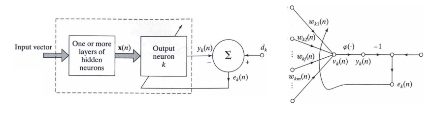
• input $x(n)$, output $y_k(n)$ and desired response or target output $d_k(n)$
• error signal $e_k(n) = d_k(n) - y_k(n)$
• $e_k(n)$ actuates a control mechanism that gradually adjust the synaptic weights, to minimize the cost function (or index of performance)
  • cost function: $\epsilon(n) = 0.5 e_k^2(n)$

• when synaptic weights reach a steady state, learning is stopped.

• Widrow-Hoff rule, with learning rate $\eta$:
  • $$\Delta w_{kj}(n) = \eta e_k(n) x_j(n)$$
• With that, we can update the weights:
  • $$w_{kj}(n+1) = w_{kj}(n)+\Delta w_{kj}(n)$$

memory-based learning

• All (or most) past experiences are explicitly stored, as input-target pairs $\{(x_i,d_i)\}_{i=1}^{N}$
• Two classes $C_1,C_2$
• Given a new input $x_{test}$, determine class based on local neighborhood of $x_{test}$.
  • Criterion used for determining the neighborhood
  • Learning rule applied to the neighborhood of the input, within the set of training examples.

nearest neighbor

Nearest neighbor $x'_N \in X$ of $x_{test}$:
\[min_i d(x_i,x_{test}) = d(x_N’,x_{test})\]
where $d(a,b)$ is the Euclidean distance.

• $x_{test}$ is classified as the same class as $x'_N$

k-nearest neighbor

• Identify k classified patterns that lie nearest to the test vector $x_{test}$, for some integer k.
• Assign $x_{test}$ to the class that is most frequently represented by the k neighbors (use majority vote)
• In effect, it is like averaging. It can deal with outliers

Hebbian Learning

• If two neurons on either side of a synapse are activated simultaneously, the synapse is strengthened.
• If they are activate asynchronously, the synapse is weekened or eliminated.

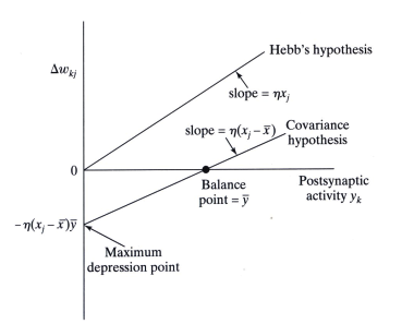
Hebbian learning with learning rate $\eta$: $\Delta w_{kj}(n) = \eta y_k (n) x_j (n)$
Covariance rule: $\Delta w_{kj}(n) = \eta (y_k - \bar{y}) ( x_j - \bar{x})$

covariance rule

• convergence to a nontrivial state
• prediction of both potentiation and depression
• observations
  • weight enhanced when both pre- and post-synaptic activities are above average
  • weight depressed when
    • pre- more than average, post- less than average
    • pre- less than average, post- more than average

competitive learning

• Output neurons compete with each other for a chance to become active.
• Highly suited to discover statistically salient features (that may aid in classification)
• three basic elements:
  • Same type of neurons with different weight sets, so that they respond differently to a given set of inputs
  • A limit imposed on strength of each neuron
  • Competition mechanism, to choose one winner: winner-takes-all neuron.

\[\Delta w_{kj} = \eta (x_j-w_{kj}), \mbox{ if } k \mbox{ is the winner}\]

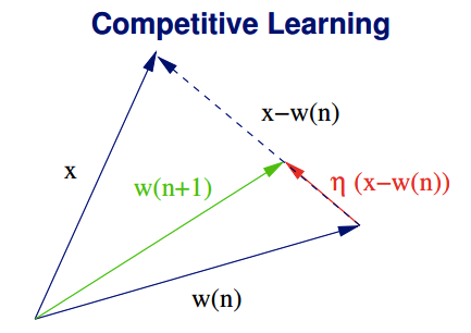
Synaptic weight vector is moved toward the input vector.
Weight vectors converge toward local input clusters: clustering

Boltzmann Learning

• Stochastic learning algorithm rooted in statistical mechanics
• Recurrent network, binary neurons (+1 or -1)
• Energy function $E = -0.5\sum_{j}\sum_{k,k \ne j} w_{kj} x_k x_j$
• Activation:
  • Choose a random neuron k
  • Flip state with a probability (given temperature T)
    • \[P(x_k \rightarrow -x_k) = (1+exp(-\Delta E_k/T))^{-1}\]
    • $\Delta E_k$ is the change in E due to the flip

Boltzmann Machine

Types of neurons

• Visible: can be affected by the environment
• Hidden: isolated

Types of operations

• Clamped: visible neurons are fixed by environmental input and held constant

• Free-running: all neurons update their activity freely.

• Learning
  • update weight during both clamped and free running condition
• Train weight $w_{kj}$ with various clamping input patterns
• After training is completed, present new clamping input pattern that is a partial input of one of the known vectors
• Let it run clamped on the new input (subset of visible neurons), and eventually it will complete the pattern

Learning Paradigms

credit assignment

Assign credit or blame for overall outcome to individual decisions.

• for outcomes of actions
• for actions to internal decisions

learning with a teacher

learning without a teacher

two classes

• reinforcement learning/neurodynamic programming
• unsupervised learning/self-organization

reinforcement

Goal is optimize the cumulative cost of actions.
In many cases, learning is under delayed reinforcement.

unsupervised

Based on task-independent measure

learning tasks, memory and adaptation

pattern association

Associate key pattern with memorized pattern.

pattern classification

Mapping between input pattern and a prescribled number of classes.

function approximation

Nolinear input-output mapping.
System identification: learn function of an unknown system

control

Control a plant, adjust plant input u so that the output of the plant y tracks the reference signal d.

filtering/beamforming

Filtering: estimate quantity at time n, based on measurements up to time n
smoothing: estimate quantity at time n, based on measurements up to time n+a
prediction: estimate quantity at time n+a, based on measurements up to time n

memory

q pattern pairs $(x_k,y_k)$:
Input (key) vector: $x_k$
Output (memorized) vector: $y_k$
By a weight matrix:
\[y_k = W(k)x_k\]

Let
\[M = \sum_{k=1}^{q} W(k)=\sum_{k=1}^{q} y_k x_k^T\]
If all $x_k$ are nomalized to length 1, then:
\[M x_j = y_j\]

adaptation

• stationary environment: supervised learning can be used to obtain a relatively stable set of parameters
• nonstationary environment: parameters need to be adapted over time
• locally stationary

statistical nature of learning

Target function: $f(x)$

Neural network realization of the function: $F(x,w)$ or $F(x,T)$

Random input vectors $X \in \{x_i\}_{i=1}^N$ and random output scalar values $D \in \{d_i\} _{i=1}^N$

Training set: $T=\{(x_i,d_i)\}_{i=1}^{N}$

regressive model: $D = f(X) + \epsilon$

Error term has zero mean: $E[\epsilon \vert x] = 0$

\[E[D \vert x] = f(x)\]

\[E[\epsilon f(X)] = 0\]

Cost function:
\[\mathcal{E}(w)= \frac{1}{2}\sum_{i=1}^{N}(d_i - F(x_i,w))^2\]
\[\mathcal{E}(w)= \frac{1}{2}E_T[\epsilon^2] + E_T[\epsilon(f(x)-F(x,T))]+\frac{1}{2}E_T[(f(x)-F(x,T))^2]\]

The first term is intrinsic error; second reduces to 0; we are interested in the third term.

bias and variance

• bias: how much $F(x,T)$ differs from the true function $f(x)$, approximation error
• variance: the variance in $F(x,T)$ over entire training set $T$, estimation error

VC dimension

Vapnik-Chervonenkis

Shattering: a dichotomy of a set S is a partition of S into two disjoint subsets.

A set of instances S is shattered by a function class $\mathcal{F}$ if and only if for every dichotomy of S there exists some function in $\mathcal{F}$ consistent with this dichotomy.

The VC dimension is the size of the largest finite subset shattered by that function.

At least one subset of a size can be shattered, then this size can be shattered by that $\mathcal{F}$.

If $\mathcal{F}$ is a set of lines, $VC(\mathcal{F}) = 3$

VC dimension increases:

• Training error decreases
• confidence interval increases
• sample complexity increases