
B+ tree 0919
- A popular data structure used in database, dealing with data stored in disks.
- Support fast search
- Support dynamic changes
- Support range search
Node
A node of order n has:
- n keys: search-keys (values of the attributes in the index)
- n+1 pointers (disk address)
Basically we want each B+ treenode to fit in a disk block so that a B+ treenode can be read/written by a single disk I/O. Typically, n ~ 100-200.
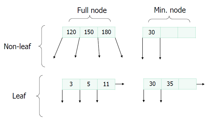
To keep the nodes not too empty, also for the operations to be applied efficiently: Basically, use at least one half of the pointers
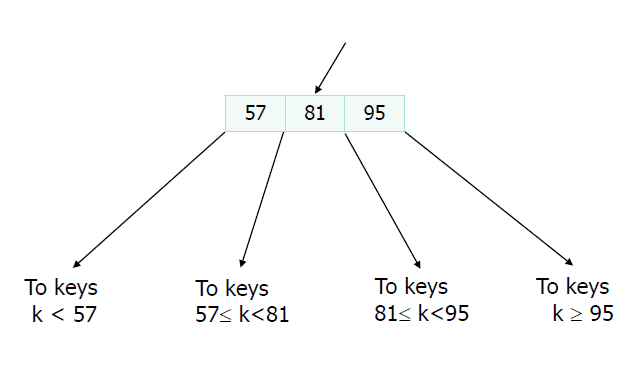
- Non-leaf:
at least (n+1)/2 pointers (to children) - Leaf:
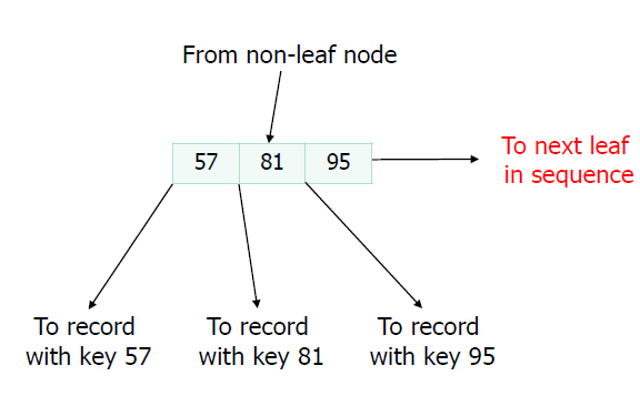
at least (n+1)/2 pointers to data (plus a “sequence pointer” to the next leaf)
A sample non-leaf with n = 3 is as
A sample leaf with n = 3 is as
Example for full and min node with n = 3 is as
Rules
- All leaves are at same lowest level (balanced tree)
- Pointers in leaves point to records except for “sequence pointer”
- Number of keys/pointers in nodes:
| Type | Max. No. pointers | Max. No. keys | Min. No. pointers | Min. No. keys |
|---|---|---|---|---|
| Non-leaf | n+1 | n | (n+1)/2 | (n+1)/2 - 1 |
| Leaf | n+1 | n | (n+1)/2 + 1 | (n+1)/2 |
| Root | n+1 | n | 2 or 1 | 1 |
Search
Search(ptr, k);
\\search a record of key value in the subtree rooted at ptr
\\assume the B+tree is a dense index of order
CASE 1. is a leaf\\is the sequence pointerIF () for a key in *ptr THEN RETURN ;
ELSE RETURN Null;CASE 2. is not a leaf
find a key in *ptr such that ;
RETURN Search(, );
Range search
To research all records whose key values are between and :
Range-Search(, , )
- Call Search(, ) to find the leaf of value ;
- Follow the sequence pointers until the search key value is larger than .
Insert
- Find the leaf L where the record r should be inserted;
- If L has further room, then insert r into L, and return;
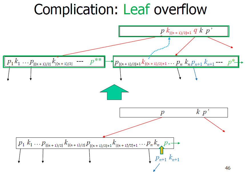
- If L is full, spilt L plus r into two leaves (each is about half full): this causes an additional child for the parent P of L, thus we need to add a child to P;
- If P is already full, then we have to split P and add an additional child to P’s parent … (recursively)
Leaf overflow
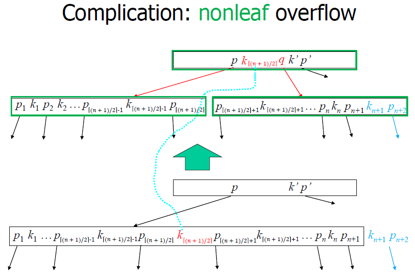
Non-leaf overflow
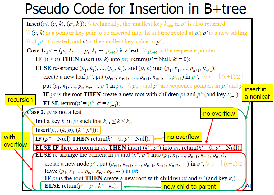
Pseudo Code
Leaf part:
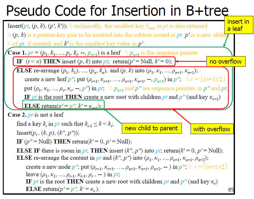
Non-leaf part
Delete
- Find the leaf L where the record r should be deleted;
- If L remains at least half-full after deleting r, then delete r, and return;
- Else consider the sibling L’ of L;
- If L’ is more than half-full, then move a record from L’ to L, and return;
- Else combine L and L’ into a single leaf;
- But now you need to consider the case of deleting a child from L’s parent … (recursively)
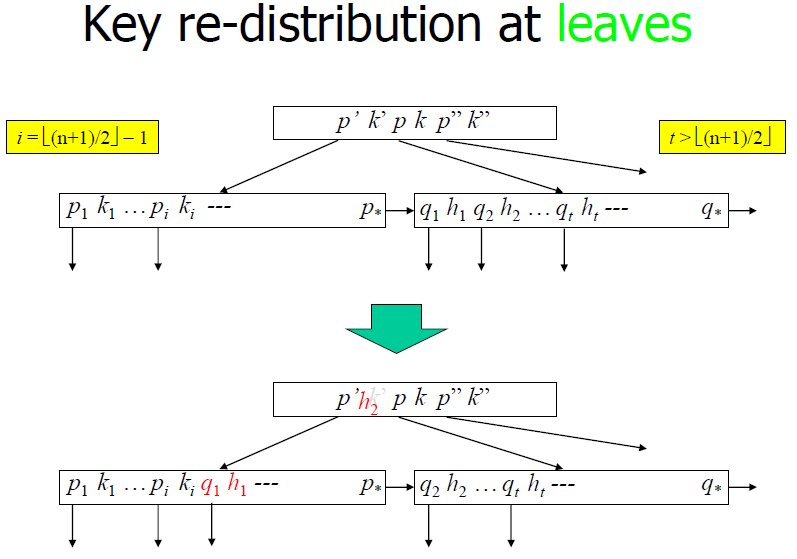
Key re-distribution at leaves
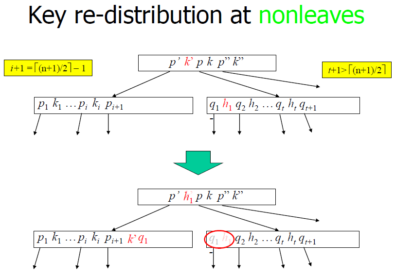
Key re-distribution at nonleaves
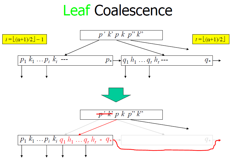
Leaf coalescence
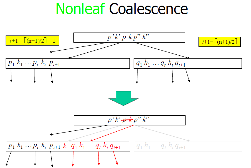
Non-leaf coalescence
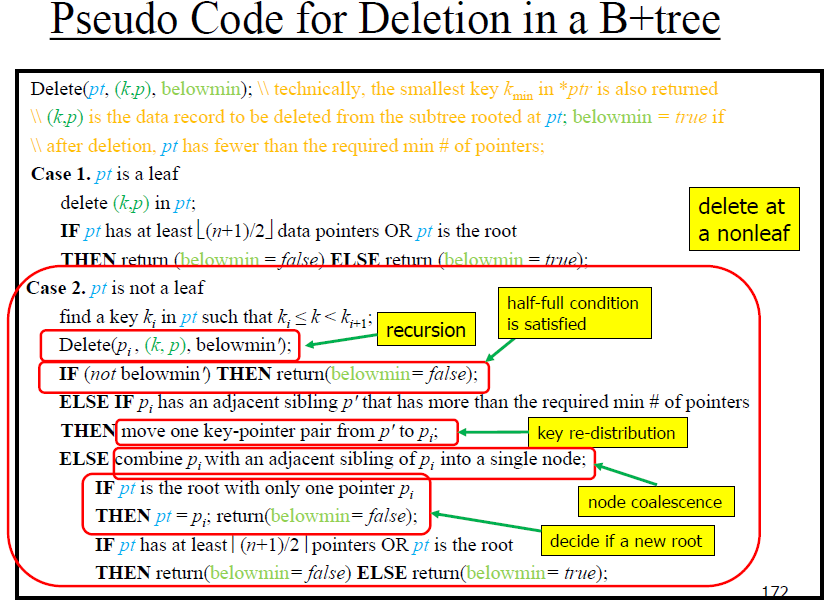
Pseudo Code
Practice
Often, coalescing is not implemented. Too hard and not worth it!
Elevator Algorithm 0921
To process disk request, but not the optimal algorithm.
The basic idea is keep going & process request until no request, then reverse direction.
Algorithm
- dir: up, down, stop
- UQ: upper queue
- LQ: lower queue
- pos: postion of the processor
PROCESS()
- IF UQ is empty and LQ is empty
THEN dir = stop; RETURN- IF dir = up
THENIF UQ is not empty
THEN x = MIN(UQ); pos = x; DELETE(UQ, x);
ELSE IF LQ is not empty
THEN dir = down
ELSEdir = stop; RETURN
ELSE
\\dir = down
IF LQ is not empty
THEN x = MAX(LQ); pos = x; DELETE(LQ, x)
ELSE IF UQ is not empty
THEN dir = up
ELSEdir = stop; RETURN;
REQUEST(x)
- IF x > pos
THEN INSERT(UQ, x)
ELSE INSERT(LQ, x)- IF dir = stop
THEN activate PROCESS
Segment intersection 0926
Geometric sweeping
In this notes, we illustrate a technique called geometric sweeping and use it to solve the segment intersection problem. Geometric sweeping is a generalization of a technique called plane sweeping, that is primarily used for 2-dimensional problems. In most cases, we will illustrate the technique for 2-dimensional cases. The generalization to higher dimensions is straightforward. This technique is also known as the scan-line method in computer graphics, and is used for a variety of applications, such as shading, polygon filling, among others.
The technique is intuitively simple. Suppose that we have a line in the plane. To collect the geometric information we are interested in, we slide the line in some way so that the whole plane will be “scanned” by the line. While the line is sweeping the plane, we stop at some points and update our recording. We continue this process until all interesting objects are collected.
There are two basic structures associated with this technique. One is for the sweeping line status, which is an appropriate description of the relevant information of the geometric objects at the sweeping line, and the other is for the event points, which are the places we should stop and update our recording. Note that the structures may be implemented in different data structures under various situations. In general, the data structures should support efficient operations that are necessary for updating the structures while the line is sweeping the plane.
Problem
Segment Intersection. Given n line segments in the plane, find all intersections.
Assume:
- No two stop points on the same vertical line
- No vertical segment
Idea
Suppose that we have a vertical line L. We sweep the plane from left to right. At every moment, the sweeping line status contains all segments intersecting the line L, sorted by the y-coordinates of their intersecting points with L. The sweeping line status is modi ed whenever one of the following three cases occurs:
- The line L hits the left-end of a segment S. In this case, the segment S was not seen before and it may have intersections with other segments on the right side of the line L, so the segment S should be added to the sweeping line status;
- The line L hits the right-end of a segment S. In this case, the segment S cannot have any intersections with other segments on the right side of the line L, so the segment S can be deleted from the sweeping line status;
- The line L hits an intersection of two segments S1 and S2. In this case, the relative positions of the segments S1 and S2 in the sweeping line status should be swapped, since the segments in the sweeping line status are sorted by the y-coordinates of their intersection points with the line L.
It is easy to see that the sweeping line status of the line L will not be changed when it moves from left to right unless it hits either an endpoint of a segment or an intersection of two segments. Therefore, the set of event points consists of the endpoints of the given segments and the intersection points of the segments. We sort the event points by their x-coordinates.
We use two data structures EVENT and STATUS to store the event points and the sweeping line status, respectively, such that the set operations MINIMUM, INSERT, and DELETE can be performed efficiently (for example, they can be 2-3 trees). At very beginning, we suppose that the line L is far enough to the left so that no segments intersect L. At this moment, the sweeping line status is an empty set. We sort all endpoints of the segments by their x- coordinates and store them in EVENT. These are the event points at which the line L should stop and update the sweeping line status. However, the list is not complete since an intersection point of two segments should also be an event point.
Unfortunately, these points are unknown to we at beginning. For this, we update the structure EVENT in the following way. Whenever we fi nd an intersection point of two segments while the line L is sweeping the plane, we add the intersection point to EVENT. But how do we find these intersection points?
Note that if the next event point to be hit by the sweeping line L is an intersection point of two segments S1 and S2, then the segments S1 and S2 should be adjacent in the sweeping line status. Therefore, whenever we change the adjacency relation in STATUS, we check for intersection points for new adjacent segments. When the line L reaches the right-most endpoint of the segments, all possible intersection points are collected.
Algorithm
Algorithm SEGMENT-INTERSECTION
Given: n line segments S1, S2, … , Sn
Output: all intersections of these segments
Implicitly, we use a vertical line L to sweep the plane. At any moment, the segments intersecting L are stored in STATUS, sorted by the y-coordinates of their intersection points with L. The event points stored in EVENT are sorted by their x-coordinates
- Sort the endpoints of the segments and put them in EV;
- ST = ;;
- while EV do
3.1. p = MINIMUM(EV); DELETE(EV, p);
3.2. if p is a right-end of some segment S thenlet Si and Sj be the two segments adjacent to S in ST;
if p is an intersection point of S with Si or Sj then REPORT(p);
DELETE(ST, S);
if Si and Sj intersect at p1 and x(p1) x(p) then INSERT(EV, p1);3.3. else if p is a left-end of some segment S then
INSERT(ST, S);
let Si and Sj be the adjacent segments of S in ST;
if p is an intersection point of S with Si or Sj then REPORT(p);
if S intersects Si at p1 with x(p1) > x(p), INSERT(EV, p1);
if S intersects Sj at p2 with x(p2) > x(p), INSERT(EV, p2);3.4. else if p is an intersection of segments Si and Sj with Si on the left of Sj in ST then
REPORT(p);
swap the positions of Si and Sj in ST;
Let Sk be the segment left to Sj and let Sh be the segment right to Si in ST;
if Sk and Sj intersect at p1 with x(p1) > x(p) then INSERT(EV, p1);
if Sh and Si intersect at p2 with x(p2) > x(p) then INSERT(EV, p2).
Analysis
Step 1, sorting the endpoints of the segments, can be done in time . Step 2 takes constant time .
For step 3, suppose there are intersection points for these segments. In the while loop, each segment is inserted then deleted from the structure ST exactly once, and each event point is inserted then deleted from the structure EV exactly once. There are event points. If we suppose that the operations MINIMUM, INSERT, and DELETE can all be done in time on a set of elements, then processing each segment takes at most time, and processing each event point takes at most time. Therefore, the algorithm runs in time
Observe that is at most , so . Thus we conclude that the algorithm SEGMENT-INTERSECTION runs in time .
We remark that the time complexity of the above algorithm depends on the number of intersection points of the segments and the algorithm is not always efficient. For example, when the number m is of order , then the algorithm runs in time , which is even worse than the straightforward method that picks every pair of segments and computes their intersection point. On the other hand, if the number m is of order , then the algorithm runs efficiently in time .
Reference
This is my class note of CSCE 629 in Texas A&M taught by Dr. Jianer Chen. Credit to him.
