Transport-layer services

Logical communication between processes on different hosts

• TCP
  • Congestion control
  • Flow control
  • Connection setup
• UDP
  • Unreliable, unordered
• No such services
  • Delay or loss guarantees
  • Bandwidth guarantees

Multiplexing and demultiplexing

• Multiplexing at sender host
  • Gathering data from multiple sockets, enveloping data with header (later used for demultiplexing)
• Demultiplexing at receiver host
  • Delivering received segments to correct socket

UDP socket

UDP socket is identified by two-tuple: dest IP address, dest port number. Receiver uses destination port number in transport header to direct the package to appropriate socket (if the socket is open).

TCP socket

TCP socket is identified by following 4-tuple. Receiver host uses all four values to direct segment to appropriate socket.

• Source IP address
• Source port number
• Destination IP address
• Destination port number

Server host may support many simultaneous TCP sockets on same port, e.g., web server on port 80.

Connectionless transport: UDP

• Best-effort service
• Connectionless
• Often used for streaming multimedia
• DNS

Advantages:

• Less overhead, no connection or retransmission
• Simplicity: no connection state at sender/receiver
• Small segment header
• No congestion control
  • For short transfers, this is completely unnecessary
  • In other cases, desirable to control rate directly from application

Packet format:

// 32 bits for a line
source port, dest port
length, checksum
// begin of message
data 

Principles of reliable data transfer

Stop-and-wait

• rdt1.0
  • Assumption
    • No bit errors
    • No loss of packets
    • No reordering
  • Simple
  • Send and receive
• rdt2.0
  • May have bit errors
  • Receiver sends ACKs or NAKs back
  • Sender may retransmit
  • Problem: ACKs and NAKs may corrupt
• rdt2.1
  • Handles garbled ACK/ NAKs
  • Add sequence number to packet (0 and 1)
• rdt2.2
  • Use ACKs only
  • ACKs contains the sequence number of packet being ACKed
• rdt3.0
  • Add retransmit when timeout

The link utilization of rdt3.0 is low. We can improve it by pipelining, sending multiple unACK’ed packets at any time.

Go-back-N

• Window of up to N consecutive unack’ed pkts allowed
• A field in header that holds k unique seq numbers
  • Maximum window size is k - 1
• ACK(n): ACKs all consecutive pkts up to & including seq # n (cumulative ACK)
  • Means packets 1…n have been delivered to application
• Timer for the oldest unacknowledged pkt (send_base)
  • Upon timeout: retransmit all sent pkts in current window (start from send_base ); reset the timer
• ACK-only: Receiver always sends ACK for correctly-received pkt with highest in-order seq #
  • Duplicate ACKs during loss
  • Need only remember expectedseqnum
• Out-of-order pkt
  • Discard, no receiver buffering!
  • Re-ACK pkt with highest in-order seq #

Selective repeat

• Receiver individually acknowledges all correctly received pkts
  • Buffers pkts, as needed, for eventual in-order delivery to upper layer
• Sender only resends pkts for which ACK was not received
  • Separate timer for each unACKed pkt
• Sender window
  • N consecutive packets in [snd_base, snd_base+N-1]
• The maximum window size is half of the sequence number range

Connection-oriented transport: TCP

• Point-to-point (unicast)
• Reliable, in-order byte stream
  • Packet boundaries are not visible to the application
• Pipelined
  • TCP congestion and flow control set window size
• Send & receive buffers
• Full duplex data
  • Bi-directional data flow in same connection
• Connection-oriented
  • Handshaking
• Flow control
  • Sender will not overwhelm receiver

TCP segment format is as below.

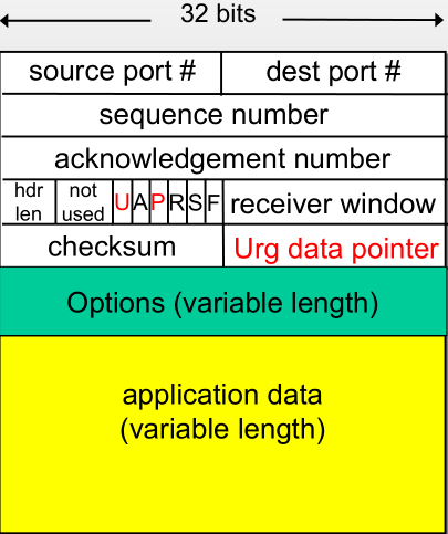
• Sequence number is the number of first byte of the segment’s data
• ACK number is the number of next byte expected

TCP RTO

• RTO (timeout value) is estimated based on history RTTs (round trip time).
• SampleRTT: measured time from segment transmission until ACK receipt
  • Ignore retransmissions to avoid inaccurate measurements
• Exponentially weighted moving average (EWMA)
  • Influence of past sample decreases exponentially fast
  • Typical value: $\alpha = 1/8$, $\beta = 1/4$

Estimated RTT:

Dev RTT:

Final RTO:

TCP Reliable Data Transfer

• TCP creates rdt service on top of IP’s unreliable service
  • Hybrid of Go-back-N and Selective Repeat
• Pipelined segments
• Cumulative acks
• TCP uses single retransmission timer
  • For the oldest unACK’ed packet
• Retransmissions are triggered by
  • Timeout events
  • Duplicate acks for base (3 in row), fast retransmission
• Nagle’s algorithm
  • For in-order arrival of packets, send ACKs for every pair of segments; if second segment of a pair not received in 500ms, ACK the first one alone
• Fast retransmit
  • If sender receives 3 duplicate ACKs for its base, it assumes this packet was lost
  • Resend the base segment immediately (i.e., without waiting for RTO)
  • Reordering may trigger unnecessary retx
  • To combat this problem, modern routers avoid load-balancing packets of same flow along multiple paths

TCP flow control

Sender won’t overflow receiver buffer by transmitting too much, too fast

• Receiver advertises spare room by including value of RcvWin in segments
  • RcvWin = RcvBuffer – [LastByteReceivedInOrder - LastByteDelivered]
• Sender enforces seq < ACK + RcvWin
• Combining both constraints (sender, receiver)
  • seq < min(sndBase+sndWin, ACK+RcvWin)

TCP connection

Purpose of connection establishment:

• Exchange initial seq #s
  • Can be random picked for security
• Exchange flow control info (i.e., RcvWin)
• Negotiate options (SACK, large windows, etc.)

3-way handshake

1. Client sends TCP SYN to server
   • Specifies initial seq # X and buffer size RcvWin
   • No data, ACK = 0
2. Server gets SYN, replies with SYN+ACK
   • Sends server initial seq # Y and buffer size RcvWin
   • No data, ACK = X+1
3. Client receives SYN+ACK, replies with ACK segment
   • Seq = X+1, ACK = Y+1
   • May contain regular data, but many servers will break
4. regular packets
   • Seq = X+1, ACK = Y+1

4-way bye-bye

• TCP initiates a close when it has all ACKs for the transmitted data
• To close a connection like closesocket(sock);, birectional transfer means both sides must agree to close.

1. Originator end system sends TCP FIN control segment to server
   • Server may issue FIN as well
2. Other side receives FIN, replies with ACK. Connection in “closing” state. Then sends FIN
3. Originator receives FIN, replies with ACK
   • Enters “timed wait” - will respond with ACK to received FINs
4. Other side receives ACK; its connection considered closed
5. after a timeout (TIME_WAIT state lasts 240 seconds), originator’s connection is closed as well

TCP congestion control

Congestion is the case when too many sources sending too much data too fast for the network to handle, not the receiver (in the case of flow control).

Manifestations:

• Lost packets (buffer overflows)
• Delays (queueing in routers)

Approaches Towards Congestion Control

• End-to-end
  • No explicit feedback from network
  • Congestion inferred by end-systems from observed loss/delay
  • TCP
• Network-assisted
  • Routers provide feedback to end systems
  • ATM (2 bits)
  • 3 states: Increase, decrease, hold steady
  • Use RM (resource management) packets, sent by sender

TCP congestion control

Various of algorithms have been developed over the years.

• TCP Tahoe (1988)
• TCP Reno (1990)
• …
• Linux 2.6.8 and later: BIC TCP (2004)
• Vista and later: Compound TCP (2005)

Idea

• Sender limits transmission by: $LastByteSent - LastByteAcked \le CongWin$.
• $CongWin$ is a function of network congestion.
• The effective window is the minimum of CongWin, flow-control window and sender’s buffer space.
• Loss event is either timeout or 3 duplicate ACKs.
• TCP sender will reduce $CongWin$ after lost event

Mechanisms

• AIMD (congestion avoidance)
  • Add 1 packet to window size per RTT
• Slow start
  • Add 1 packet to window size per ACK; double W per RTT
• Conservative after timeout events

Refinement

TCP Tahoe only responds to timeouts.

• Reset: $Threshold = CongWin / 2$
• $CongWin$ is set to 1 MSS
• Slow start until $Threshold$ is reached, then AIMD

TCP Reno:

• Timeouts same as Tahoe
• 3 dup ACKs:
  • $CongWin$ cut in half
  • AMID

Initial slow start ends when either:

• Loss occurs
• Initial threshold is reached
  • Usually set to the receiver’s advertised window

Transfer rate

Rate is $W * MSS/ RTT$, $W$ is the current window size. Average rate is $0.75 * W_{max} * MSS/ RTT$.

Between two losses, number of packets sent is:

Denote loss probability is $p$, Therefore, we have:

The average rate can be calculated again to be:

TCP Fairness

Fairness goal: if K TCP sessions share same bottleneck link of bandwidth C, each should have average rate of C/K.

TCP will converge to fairness eventually, in the case that flows have the same MSS/RTT.

Nothing prevents app from opening parallel flows between 2 hosts. Can use this strategy to obtain larger share of bandwidth. Web browsers do this.

Multimedia apps do not use TCP; they use UDP instead. Because they don’t want rate throttled by congestion control.

Reference

This is my class notes while taking CSCE 612 at TAMU. Credit to the instructor Dr. Loguinov.