Reference

Link to paper

Abstract

• Distributed relational database
• Filial 1 hybrid, of
  • System community: high availability, scalability.
  • Database community: consistency and usability.
    • SQL query, automatic change tracking and publishing.
• On Spanner: synchronous replication and strong consistency.
  • Higher commit latency
• Mitigate high latency
  • Hierarchical schema model with structured types.
  • Smart application design.

Introduction

• Both OLTP and OLAP database for AdWords system.
  • Adwords as of 2013:
    • 100s applications; 1,000s users
    • 100TB data
    • ~1M QPS
    • SQL queries scan O(10^13) rows per day.
    • Availability: 99.999%
    • Not higher latency compared with the old MySQL backend.
  • Some other applications use it as well.
• Built to replace old MySQL backend.

Key goals of F1’s design are as below. These goals are mutually exclusive, but F1 achieved them with trade-offs and sacrifices.

• Scalability
  • Scale up trivially and transparently.
• Availability
  • Must never go down for any reason.
• Consistency
  • ACID transactions.
• Usability
  • SQL query and other SQL features like indexes and ad hoc query.

F1 inherits features from Spanner and adds more:

• Distributed SQL queries
• Transactionally consistent 2nd indexes
• Asynchronous schema changes
• Optimistic transactions
• Automatic change recording and publishing

To hide the high latency brought by the design, some techniques are developed:

• F1 schema makes data clustering explicit.
  • Using hierarchical relationships and columns with structured data types.
  • Result: Improve data locality; reduce number of internal RPCs to read remote data.
• F1 users heavily use batching, parallelism and asynchronous reads.
  • A new ORM (object-relational mapping) library makes these explicit.

Basic architecture

F1 architecture:

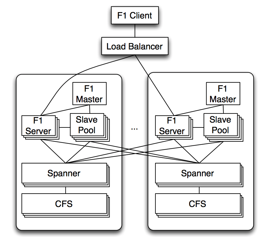
• F1 severs: receives clients’ read and write requests.
  • Load balancer may choose a server far away from clients in cases of high load or failures.
  • F1 servers usually co-locate with Spanner servers, but may contact other Spanner servers when necessary.
  • F1 servers are usually stateless, unless a pessimistic transaction is in process and server must hold locks.
    • A client can contact different servers for different requests.
  • Servers can be quickly added or removed and require no data movement.
    • Adding or removing Spanner servers requires data movement but the process is transparent to F1.
• Slave pool: for distributed SQL queries.
  • Distributed execution is chosen when the query planner finds that increased parallelism will reduce latency.
• F1 master: manage the membership of slave pool.
• Support MapReduce framework, talking to Spanner directly.

With this architecture, throughput can be scaled up by adding more Spanner servers, F1 servers or F1 slaves. Since the servers are widely distributed, the commit latencies are relatively high (50 - 150 ms).

Spanner

Check out this note.

Data model

Hierarchical schema

Originally, Spanner used a Bigtable-like model; but later Spanner actually adopts the hierarchical logical data model of F1. (Directory table, child tables, etc) F1 schema supports explicit table hierarchy and columns with Protocol Buffer data types.

• Child tables are clustered with and interleaved within the rows from its parent table.
• Child and grand child table share the same primary key prefix with the root table row.
• A root row in root table and its hierarchy form a Spanner directory.
  • In F1, make Customer (Advertiser) a root table.
• Child rows are stored under their parent row ordered by primary key.

Hierarchy example:

Customer 1
  Campaign 1 1
    Ads 1 1 1 
    Ads 1 1 2
  Campaign 1 2 (interleaved; doesn't stay next to Campaign 1 1)
    Ads 1 2 1
Customer 2
  ...

Advantages:

• Can fetch Campaign and Ads records (without knowing the Campaign ID) in parallel.
• Use a single range read to get all Ads under a Customer.
  • Don’t need indexes.
• Since records are ordered, can join two tables with a simple ordered merge.
• Reduce the number of Spanner groups involved in a transaction.
  • Application developers should try to use single-root transaction as much as possible.
    • If must use multiple roots, we should limit the number of roots involved to reduce 2PC cost.

Protocol buffers

• Columns can be Protocol buffers, a structured data type.
• Can use it across storage and code.
• repeated fields can be used to replace child tables.
  • Number of records in a such field is limited.
  • Reduce overhead and complexity to store and join child tables.
  • Easier for users to use the object as an atomic unit.

A single protobuf column or multiple columns?

• Many tables consist of a single protobuf column.
• Others has multiple columns.
  • Split by:
    • grouping fields usually accessed together.
    • static vs. frequently updated data.
    • different read/write permissions.
  • Allows concurrent updates to different columns.
• Using fewer columns generally reduces performance overhead.

Indexing

• All indexes are transactional and fully consistent.
• Store: index key -> primary key of the indexed table.
  • Type:
    • Local
      • The index key contains the root row primary key as a prefix.
      • Stored in the same directory as the root row.
      • Updating cost is little.
    • Global
      • The index key doesn’t contain the root row primary key.
      • Updating is often large and rate is high.
        • Thus sharded into many directories.
      • Use it sparingly due to its cost and try to use small transaction if must do it.

Schema changes

AdWords system requires F1 to be highly available; schema changes should not lead to downtime or table locking.

Challenges:

• Servers distributed in multiple geographic regions.
• F1 servers have schema loaded in memory; not practical to update atomically across all servers.
• Queries and transactions must continue on all tables even with ongoing schema changes.
• Schema changes should not impact availability and latency.

F1 chooses to do schema changes asynchronously. Servers may update the database using different schema. Note: Why not using Spanner style? Assign a future timestamp to the change. Maybe because it will block some transactions requiring the new change.

Problem: If two F1 servers update the database with different schemas (not compatible), it will lead to anomalies like data corruption.

Example of data corruption: A schema change from schema S1 to S2, adding a new index I on table T.

• Server M1 uses S1; M2 uses S2.
• M2 inserts a new row r, and adding index Ir.
• M1 deletes row r, leaving index Ir alone since it is not aware of it.
• Index scan on I will return spurious data on r.

Algorithm to prevent such anomalies:

• Enforce that at most two schemas are active across all servers.
• Subdividing each schema change into multiple phases where consecutive ones are mutually compatible and cannot cause anomalies.

The example can be divided as:

1. Add index I and only allows delete operations on it.
2. Upgrade I to allow write operations on it.
3. Perform Offline job to backfill index entries to all rows.
   • Need to carefully handle concurrent writes.
4. Once completed, make I visible to all read operations.

Full details are in this paper (Online, asynchronous schema change in F1).

Transactions

F1 must provide ACID transaction feature. In contrast, eventual consistent systems add a lot of burden on application developers. We should support full transactional consistency at database level.

3 types of F1 transactions:

• Snapshot transaction
  • Read-only
  • Use Spanner snapshot timestamp.
  • Default current (when timestamp is not provided)
• Pessimistic transaction
  • Map to Spanner transactions,
  • Can use shared or exclusive locks.
• Optimistic transaction
  • Use last modification timestamp (LMT) on each row, stored in a hidden lock column.
    • Updated in every F1 writes.
  • Check the LMT of all already read rows while trying to commit.
  • Default in F1.

Advantages of optimistic transactions:

• Tolerate misbehaved clients since not holding locks.
• Support long-lasting transactions, e.g., with user interactions.
• Easy to retry transparently on server-side.
• Client can retry on different F1 servers since optimistic transactions are server-stateless.
  • When servers failed or needs load balancing.
• Speculative writes.
  • Read values from outside; also requires their LMT.

Disadvantages of optimistic transactions:

• Insertion phantoms
  • LMT only exists on existing rows.
  • Can use parent-table locks to avoid this.
• Low throughput under high contention
  • When many clients update concurrently.
  • Use pessimistic ones or do batching updates.

Flexible locking granularity

• Row-level locking by default.
• Support column-level locking per row.
  • Can update different columns on one row concurrently.
• Can also selectively reduce concurrency.
  • Use a lock column in a parent table to cover columns in a child table.
    • Avoid insertion phantoms.

Change history

• Change history is a first-class feature and guaranteed full coverage.
• Enabled by default, but can opt out some tables or columns.

How:

• Every transaction creates one or more ChangeBatch protobuf.
  • Primary key is the root table key + transaction commit timestamp.
    • Thus is a child table of the root row, stored in commit order.
  • Stores the before and after values for each updated row.
  • If multiple root rows are involved, create the protobuf for each root row.

Applications:

• For pubsub.
• For cache.
  • If cache is stale, do incremental updating starting from the checkpoint using change history.

Client design

• Simplified ORM
  • Expose APIs for parallel and asynchronous read access.
  • Avoid anti-patterns:
    • Serial reads, implicit traversals etc.
• NoSQL interface
  • A simple KV based interface for reads/writes.
  • Can batch retrieval of rows from multiple tables in a single call.
• SQL interface
  • Supports from low-latency OLTP to large OLAP.
  • Can join data from outside sources, like Bigtable, CSV files, etc.

Query processing

Some key properties of the query processing system:

• Queries are executed as either low-latency centrally executed ones or distributed ones with high parallelism.
  • Centrally executed queries: OLTP-style.
  • Distributed queries: OLAP-style.
    • Use snapshot transactions (read-only).
• Data is remote and batching is used heavily to mitigate network latency.
  • Example: Lookup join
    • Load 50MB data from one table then lookup in the other table.
• All input and internal data is arbitrarily partitioned and has few ordering properties.
• Many hash-based repartitioning steps.
• Individual query plan operators are designed to stream data to later operators as soon as possible.
  • Thus limit the ordering properties.
  • Maximize pipelining.
  • Reduce memory usage for buffering temporary data.
• Optimized access on hierarchically clustered tables.
• Query data can be consumed in parallel.
• First-class support for structured data types, by protobuf-type columns.
• Snapshot consistency provided by Spanner.

Distributed query example

SELECT agcr.CampaignId, click.Region,
      cr.Language, SUM(click.Clicks)
FROM AdClick click
  JOIN AdGroupCreative agcr
    USING (AdGroupId, CreativeId)
  JOIN Creative cr
    USING (CustomerId, CreativeId)
WHERE click.Date = '2013-03-23'
GROUP BY agcr.CampaignId, click.Region,
        cr.Language

• AdGroup: a collection of ads with some shared configuration.
• Creative: actual ad text.
• AdGroupCreative: a table of foreign keys linking AdGroup and Creative.
• AdClick: records the AdGroup and Creative.

A possible query plan:

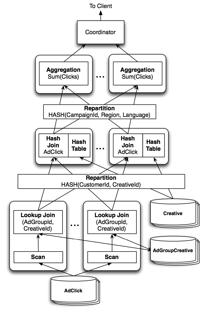
Steps:

1. Scan AdClick into a lookup join operator and do the join.
   • The operator looks up AdGroupCreative using secondary index key.
2. Repartition data stream by hashing with CustomerId and CreativeId.
3. Distributed hash join with Creative using the same keys.
4. Repartition again by hashing with GROUP BY keys (CampaignId, Region, Language).
5. Aggregate using aggregation operator.

Distributed execution overview

A distributed query plan may consist of tens of plan parts, forming a directed acyclic graph. The data flows up from the leaves to a single root node (query coordinator). Query coordinator is the server which received the initial request; it plans the execution and processes results to return to the client.

Co-partitioning of the stored data is helpful to push down large amount of query processing to nodes hosting the partitions. F1 cannot utilize this since all data are remote and Spanner does random partitioning. To allow efficient processing, F1 re-partitions data (hash partition). It requires heavy network traffic and hence limits the size of F1 cluster due to the network switch hardware. However, both are not causing problems.

F1 operators execute in memory without checkpointing, stream results as much as possible. Therefore, a single server failure will fail entire query.

Hierarchical table joins

Child table entries are interleaved in the parent table; thus a single Spanner request can work to join a parent table with its child table. Cluster join (like merge join) is efficient, which buffers one parent entry and one child entry.

Parent(3)
  Child1(3, 1)
  Child1(3, 2)
Parent(4)
  Child1(4, 1)

However, a single Spanner request doesn’t work to join two sibling child tables. (Note: How are sibling child tables interleaved in parent table?) Need to perform one cluster join first (Parent, Child1), then another join (join1 result, Child2? What primary key to use? parent root key?).

Partitioned customers

• A single query coordinator or a single client process may be a bottleneck.
  • It may receive results from many servers in parallel.
• Clients can ask F1 for distributed data retrieval.
  • F1 returns a set of endpoints to connect to.
  • A slow reader may block entire processing.
    • F1 processes results for all readers in lock-step.

Queries with protobuf

• protobuf can be used in F1 SQL path expressions like WHERE c.Info.country_code = 'US'.
• F1 can query and pass entire protobuf like SELECT c.Info
• Can access repeated fields with implicit join PROTO JOIN.
• Disadvantages:
  • Performance implications due to fetching and parsing entire protobuf, even if we only need one field.
    • Can improve by pushing the parsing and field selection to Spanner.

Deployment

• 5 datacenters across mainland US.
  • 5-way Paxos replication.
    • 3-way is not enough: If one failed, a single machine failure may fail the second one then the system is unavailable.
• Additional read-only replicas for snapshot reads.
• Put clients with heavy modifications near leaders.
  • User transactions require at least 2 round trips to the leader.
    • One for read, one for commit.
    • Maybe another read as part of a transaction commit.
• 2 at east coast; 2 at west coast; 1 centrally.
  • Leader at east cost.
    • Round trip to the other datacenter at east cost and central one accounts for 50 ms minimum latency.
      • Paxos voting process is improved since majority 3/5 is required.

Latency and throughput

• Read latencies: 5-10 ms.
• Commit latencies: 50-150 ms.
• Multi-group transaction latencies: 100-300 ms since requiring 2PC.
• User-facing latencies for AdWords interactive application: 200 ms.
  • Achieved much by avoiding serial reads.
  • Tail latencies are much better than MySQL.
• Non-interactive bulk updates:
  • Optimize for throughput instead of latency.
  • Do small transactions (only one directory involved) in parallel.
• Query processing can be speeded up linearly with more resources.
• Resource cost: CPU 1 order higher than MySQL
  • Need to decompress disk data, process then recompress and send over the network.

Related work

• Hybrid of relational and NoSQL.
• Optimistic transactions.
• Asynchrony in query processing.
• MDCC (Multi-datacenter consistency) Paxos optimizations.
• Protocol Buffers.

Conclusion

• Highly scalable, available.
• High throughput.
• ACID transactional guarantee.
• SQL query.
• Rich column types (protobuf).