
Introduction
This is a group project developed by Jimin Wen and me.
This project is to implement a Tiny-SQL interpreter. It is written in Java. In this report, first, the software architecture of this database management system is introduced; second, various optimization techniques implemented are illustrated; third, results and performance for experiments on the two test files are discussed. The first test file is the one included in the course project resources and the other is more realistic data from our course project 1. This program is able to perform basic SQL commands based on TinySQL grammar defined by the project introduction. Data structures such as heap, expression tree are created for sorting and expression evaluations. Algorithms like one-pass, two-pass are also implemented for specific usage. Furthermore, optimization techniques for select attributes push-down, natural join and table reordering based on size for join operation are also introduced in this program in order to speed up the execution.
The project code can be found at https://github.com/melonskin/tinySQL.
Run
The program has been compiled with Maven. To run the program, just cd to the project folder and type following command:
java -jar tinySQL-1.0-SNAPSHOT-jar-with-dependencies.jar
Software architecture
User interface
The overall software architecture of this database management system consists of an user interface, a parser, physical query module and storage manager and other helper modules for internal processing. The logic query discussed in the textbook is not explicitly implemented as a module and instead, the logics are implemented in those internal modules.
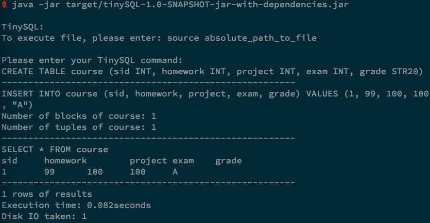
The text interface used in our program is a command line tool able to take user TinySQL command in and process the SQL command and print the results on the screen. It can also process a text file consisting of a series of tinySQL commands.
User can either choose to type the SQL command in the command line and execute the lines one by one. Or they can choose to process file input, here the command use to do a file execution is source absolute\path\to\filename.txt, in which the filename.txt is the input file to be processed, the output is directed to the screen. Notice that absolute file path is used, since it’s more flexible for users.
The UI is shown in Fig. 1.
Parser and logical query
The parser used various parser method to parse the SQL queries and output the parser tree to be executed by the physical query plan.
- The program preprocess the input query by trimming possible space at two ends.
- The program will capture the keyword of a query such as
CREATE,DROP,INSERT,SELECTandDELETE; thus to decide which parser method should be used to parse this query. - The program will use corresponding parser method to parse the query. The result is a
ParserTreecontaining all information for following execution, such as table names and attributes. An expression tree can be constructed if there is aWHEREcondition.
Expression tree
For WHERE condition, we utilize an expression tree as a data structure to store it. In order to construct the tree, we create two stack. One stack is for operator of expression tree. The other is for operands of the expression tree. Based on the TinySQL grammar provided, we first create a method to set the operator into different priority. / , * are set as 3 which is the highest level priority. Then, +, -, >, < are set as 2; = is set as 1; & which is AND is set as 0, | which is OR is set as -1. The next step is loop over the words one by one, if it is an attribute, create a new expression tree and push into the operand stack. If it is an operator, push the operator into the operator stack if the stack is empty or the existing operator’s priority is lower than the current one. If the current operator’s priority is lower than the existing one, we pop out the existing operator and pop out two operands which construct the the left child and right child of the expression tree. Then push the expression tree back to the operands stack and the tree is built recursively.
Physical query plan
CREATE, DROP and INSERT
Physical query part will take the output of the parser as its input. It includes methods for execution of DROP, CREATE, INSERT, SELECT and DELETE. For the CREATE and DROP queries, no recursion is involved in the execution, thus the implementation is pretty straightforward. Just call schemaManager to do the job.
For INSERT, new tuple is created based on the attribute values provided. It will be append the the relation then. NULL values is handled properly. There is a corner case when we need to insert the selected result from SELECT query. It can also be processed easily once we get the SELECT part done.
DELETE
Both SELECT and DELETE query can have a WHERE clause to specify the condition.
The idea of deletion is we take relation blocks in main memory. Check if the tuples inside meets the condition if there is one. Do invalidate the tuple if it satisfies the condition or there is no condition. Then put those blocks back into disk.
Notice that, the operation will create possible holes in disk. In order to handle it, the program will do two pass sort to remove holes and shrink the number of relation blocks.
SELECT
Single table
For single table case, if the query doesn’t contain DISTINCT or ORDER BY, we can just one pass to go over all tuples and filter those satisfying condition.
If we do have DISTINCT or ORDER BY, but the table size is less than or equal to the main memory capacity, we can take all tuples from disk into main memory, then do one pass sort based on order-by attributes or selected fields. Finally, output the tuples in order (remove duplicates if required).
If we do have DISTINCT or ORDER BY, but the table size is larger than the main memory capacity, we cannot put entire table into the main memory. However, we still need to sort the table. We do two pass sort based on order-by attributes or selected fields as described in class. The tuples stored in disk will be in order. Finally, output the tuples in order (remove duplicates if required).
The two pass sort algorithm is implemented by heap and merge-sort algorithm. It can also delete possible holes in disk.
Multiple tables
For multiple tables case, we need to join those tables. The basic algorithm is join two tables. Two technique are implemented: cross-join and natural join.
- Cross join: Based on the table sizes, both one pass and two pass is implemented
- one pass: If one of the table can be put into the memory, we just bring it in memory and loop over all blocks of the other table
- two pass: In this case, both tables are too large to be put into the memory. We bring several blocks of one table into the memory and loop over all blocks of the other table.
- Natural join: In this case, we join two tables based on a specific field. We first do sort to make the tuples in order of that field in the disk. Then two relation iterators are created to compare and join tuples from two tables.
Optimizations
We implement three optimization techniques to speed up the execution. The first one is pushing down the selection in the expression tree. The second strategy is to use natural join instred of cross join when applicable. The third one is reordering the tables based on table sizes while joining more than 2 tables.
- To reduce the temporary table size, first, we split the expression tree with
AND; then we push down the selection to apply them earlier in the input table. So when do later join, we only select those tuples satisfying input conditions. The temporary table size can be reduced dramatically. - Natural join is implemented when the value some fields in two tables are equal, to reduce the cost of disk IO. When more than two tables needs to be natural joined, the procedure is achieved by first joining two tables and store the temporary relation. And the relation would be utilized to join the other table. A large number of tables could be natural joined by repeating this procedure. When detecting a condition relevant to two tables that have already be natural joined. The condition would be stored to filter the natural join result.
- While joining more than two tables, we modify the join order of tables based on their sizes, like the left-deep tree problem. Those tables with smaller size will be joined first. Thus, the temporary table size will be reduced.
- While cross join multiple tables, the program will first calculate the sizes of tables, and bring as many as tables that can be fill into memory and do the join first, then perform join with remaining tables. It will reduce disk IO since it won’t create unnecessary temporary tables.
Experiments
Relation data
The sizes of the tables used in the experiment are listed as below.
| Table Name | course | course2 | r | s | t | t1 | t2 | t3 | t4 | t5 | t6 | |
|---|---|---|---|---|---|---|---|---|---|---|---|---|
| Number of tuples | 60 | 24 | 41 | 41 | 41 | 5 | 4 | 4 | 2 | 2 | 1 | |
| Number of blocks | 60 | 12 | 11 | 11 | 11 | 1 | 1 | 1 | 1 | 1 | 1 | 1 |
Natural join and Cross join
We will compare the performance of two same queries but with different join techniques, natural join and cross join. The two queries are as below. Cross join of another case is also included.
SELECT course.sid, course.grade, course2.grade FROM course, course2 WHERE course.sid = course2.sid
SELECT * FROM r, s, t WHERE r.a=t.a AND r.b=s.b AND s.c=t.c
SELECT * FROM t1, t2, t3, t4, t5, t6
| Join case | course | r, s, t | t1,t2,…,t6 |
|---|---|---|---|
| Cross join | 4767 | 21180 | 965 |
| Natural join | 502 | 364 | NA |
We can see that natural join reduces the disk IO dramatically.
Execute commands
The performance of 4 given queries is shown as below.
- Statement A:
SELECT * FROM course - Statement B:
SELECT DISTINCT * FROM course - Statement C:
SELECT grade FROM course - Statement D:
SELECT DISTINCT grade FROM course
| Command | A | B | C | D |
|---|---|---|---|---|
| Disk IO | 60 | 300 | 60 | 300 |
| Run time | 7.43 | 37.2 | 7.4 | 37.16 |
Testing data with project 1
We use a 200-tuple 3-field table from project 1 as dataset to test our program. The queries and performance are shown as below. Four statements marked as A, B, C, D were tested. The time taken and disk IO were recorded in the table below.
CREATE TABLE director (id INT,director_name STR20,director_facebook_likes INT)
INSERT INTO director (id,director_name,director_facebook_likes) VALUES (1,"James Cameron",0)
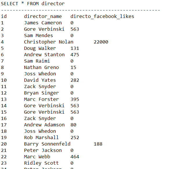
- Statement A:
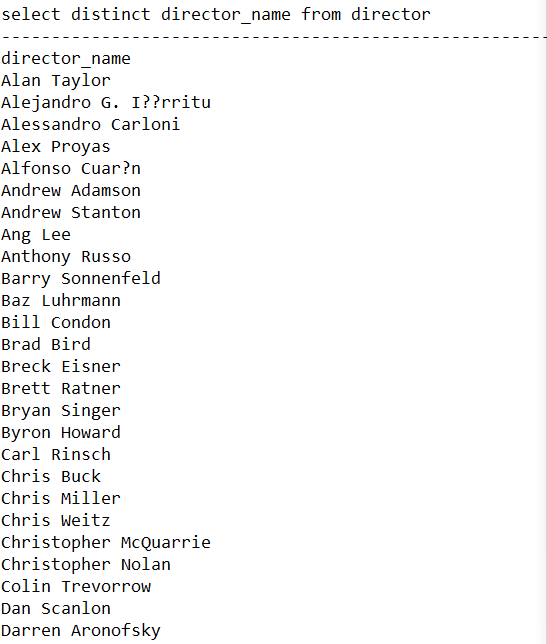
SELECT * FROM director - Statement B:
SELECT DISTINCT director_name FROM director - Statement C:
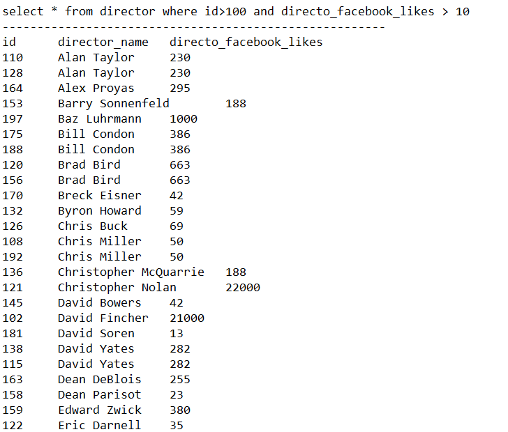
SELECT * FROM director WHERE id>100 AND director_facebook_likes > 10 - Statement D:
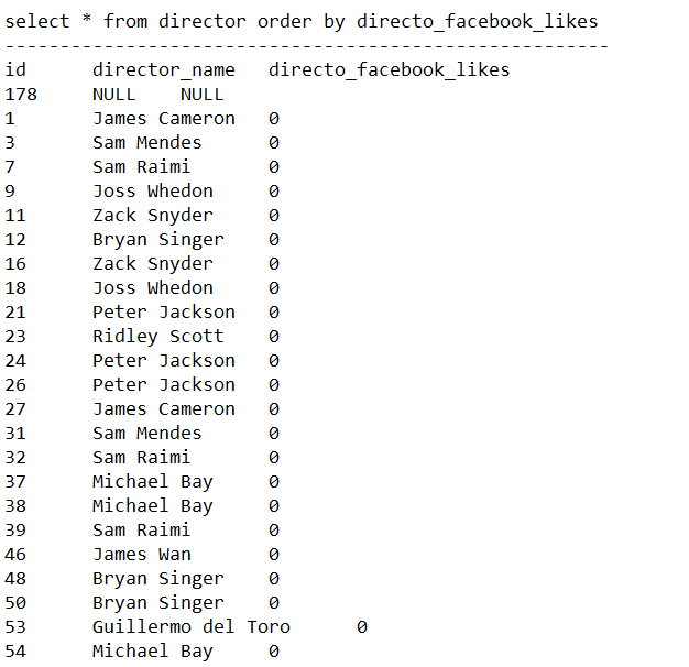
SELECT * FROM director ORDER BY director_facebook_likes
| Command | A | B | C | D |
|---|---|---|---|---|
| Disk IO | 100 | 500 | 100 | 500 |
| Result rows | 200 | 125 | 76 | 200 |
The execution results are shown in Fig.2, 3, 4, 5 as below.
To get a deeper analysis on the performance of tiny-SQL on the commands above. We tested it with increasing number of tuples and get the graph showing the change of running time and diskIO to analyze the performance.
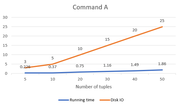
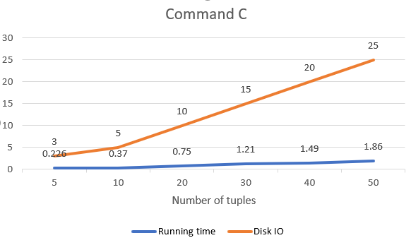
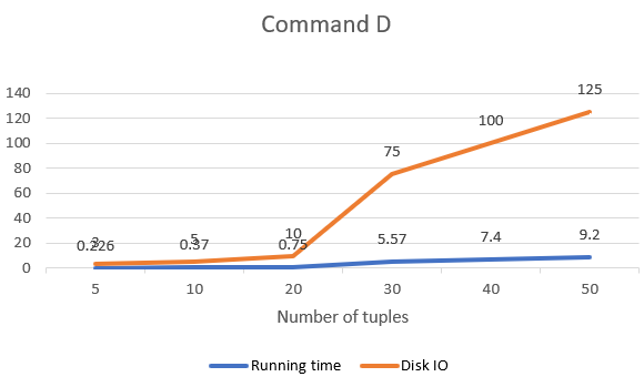
As it could be found, the graph of command A and C generally follow linear relationship. That is because A and C read in records by tuple. The cost of disk IO is linear to the number of tuples of a relationship.
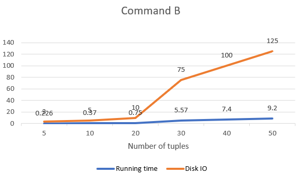
Command B and D shows a obvious steeper gradient when the number of tuples is larger than 20. That is because when the relation size is larger than the main memory. It could not be read into main memory by once when doing sorting and duplicate elimination which is based on sorting.
Conclusion
This program can execute tinySQL queries specified by tinySQL grammar provided. Various data structures and algorithms are implemented in order to perform queries, such as heap, expression tree, one pass and two pass algorithm and natural join, etc. Furthermore, two optimization techniques are applied to speed up the execution. One is to push selection down; the other is to rearrange table join order. The purpose of both techniques is to reduce the size of temporary table size.
