Introduction

• Transformer, an encoder and decoder model, solely based on attention mechanisms.
• Not using recurrence and convolutions, more parallelizable, capturing long-distance context in $O(1)$. Therefore, it requires less time to train.

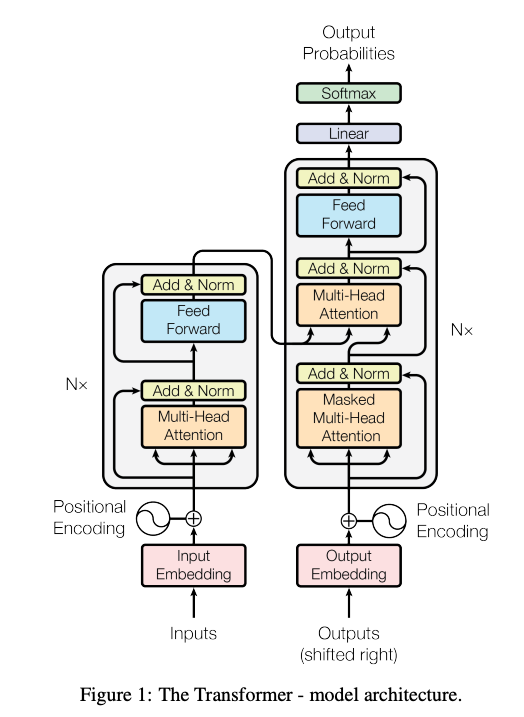
• One layer contains two sub-layers: attention and Feed Forward (FFN).
• Employ a residual connection around each of the two sub-layers, then layer normalization.
  • The output of each sub-layer is $\text{LayerNorm}(x + \text{Sublayer}(x))$
• Multiple $N$ layers. e.g., Llama-3-8B has 32 layers.

Input preparation

1. Input is a natural language sequence with $n$ tokens.
2. Input is first converted to a matrix $X$ of dimension $[n, d_{model}]$. $d_{model}$ is the dimension of token embedding vector. e.g., 768, 4096.
3. Add positional embeddings to the input matrix to provide position info for each token. The dimension doesn’t change.
   1. Using fixed sinusoid function. Can also use learned ones.

Self-attention

While processing a sequence, automatically learn the contexts, relations between different parts.

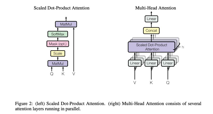
Calculate $Q$(Query), $K$(Key), $V$(Value) using the input matrix and projection matrices $W^Q, W^K, W^V$.

1. $Q = X W^Q$, the query, for each position, what context it wants to search for
   1. $W^Q$ is of dimension $[d_{model}, d_{model}]$. $Q$ is of dimension $[n, d_{model}]$.
2. $K = X W^K$, the key, for each position, what info it can provide for the search, like a search index
   1. $W^K$ is of dimension $[d_{model}, d_{model}]$. $V$ is of dimension $[n, d_{model}]$.
3. $V = X W^V$$, the value, for each position, if selected, what detailed info it can provide, like the payload
   1. $W^V$ is of dimension $[d_{model}, d_{model}]$. $V$ is of dimension $[n, d_{model}]$.

With training, $W^Q$ and $W^K$ learn about searching and matching contexts. $W^V$ learns about information providing.

\[\text{Attention}(Q, K, V) = \text{softmax}\left(\frac{QK^T}{\sqrt{d_k}}\right)V\]

1. $Q K^T$ is calculating similarity between query and all keys.
2. $\sqrt{d_k}$ is for scaling to prevent gradient vanishing.
3. Softmax is for normalizing similarity scores to probabilities, the total is 1.
4. $\times V$ gets the final value. Values with higher similarities occupy larger portion in the final value. The dimension is $[n, d_{model}]$.

Multi-head attention

Learn the same sequence from multiple aspects. Multi-head attention allows the model to learn these aspects independently, in parallel. There could be shallow heads focusing on local info, deep heads for global info.

1. Linear projection for $h$ heads: project the initial $Q, K, V$ for each head $i$ with $W_i^Q, W_i^K, W_i^V$.
   1. The dimension $d_{model}$ is usually split equally across heads. $d_h = \frac{d_{model}}{h}$. So the dimension of $QW_i^Q$ is $[n, d_h]$. So multi-head won’t increase computation cost.
2. Parallel attention: $\text(head)_i = \text(Attention)(QW_i^Q, KW_i^K, VW_i^V)$
   1. The dimension is $[n, d_h]$.
3. Concatenation: Concatenate the outputs of all heads. The dimension is $[n, d_{model}]$.
4. Final linear: use a $W^O$ to project the output back to the original dimension, also synchronize info from all heads.

• Diversity: learns in various aspects.
• Robustness: If one head fails due to noise, other heads are still working.
• Sub-space learning: Easier to capture complex info by learning in multiple lower-dimensional spaces.

Feed Forward network (FFN)

FFN is after the attention layer. It’s position/point-wise, each position only cares about itself, learning deeper information. This layer adds nonlinear to the overall model.

\[\text{FFN}\left(x\right) = \text{activation}\left(xW_1+b_1\right)W_2+b_2\]

1. Dimension expansion
   • Using $W_{up}$ of dimension $[d_{model}, d_{ff}]$ to expand the input dimension to $[n, d_{ff}]$
   • $d_{ff}$ is usually larger (~4X) than $d_{model}$. It’s easier to identify and extract complex details in higher-dimensional spaces.
2. Dimension reduction
   • Use $W_{down}$ of dimension $[d_{ff}, d_{model}]$ to reduce to the original dimension.
   • Filter noise and compress useful info.

• The activation function is nonlinear, e.g., ReLU, $MAX()$.
• Token has gained context info from attention layer; FFN is for further digesting these info.
• Dimension expansion:
• Store knowledge and memories in FFN weight matrices.
• ~2/3 weights in a LLM are in FFN.

Training

• Adam optimizer
• Regularization
  • Residual dropout on (1) the output of each sub-layer and (2) the addition of input embedding and positional embedding.
  • Label smoothing

References

• paper